A room mode calculator converts a rectangular room’s length, width, and height into a list of predicted resonant frequencies. That list is useful for finding likely bass trouble regions, especially when several modes coincide or sit close together. It does not tell you exactly how loud any frequency will be at your chair.
Quick answer: Use the calculator to form hypotheses. Look for low axial modes, frequency clusters, wide gaps, and coincident modes; then compare those frequencies with measurements at the listening positions that matter. Change speaker, subwoofer, or seat placement first, verify again, and consider equalisation or bass trapping only after geometry has been tested.
What a Room Mode Calculator Actually Calculates
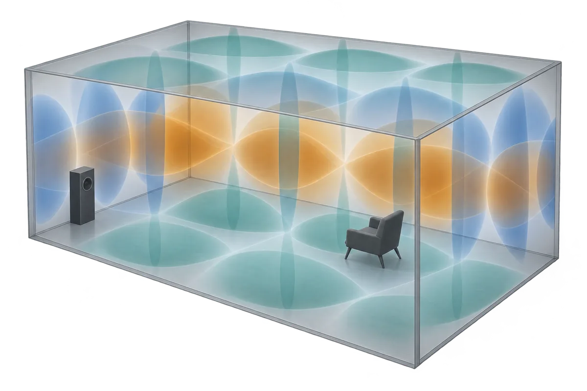
For an ideal rigid rectangular room, each mode can be labelled with three non-negative integers: (p, q, r). They describe how many half-wavelengths fit along the room’s length, width, and height. The standard relationship is:
f(p,q,r) = (c / 2) × √[(p/L)² + (q/W)² + (r/H)²]
Here, c is the speed of sound, while L, W, and H are dimensions in consistent units. Many calculators use about 343 m/s at 20°C. A small difference in temperature or measurement precision moves the prediction slightly, so a result such as 68.6 Hz should be treated as a neighbourhood, not a laboratory-perfect target.
Indiana University’s acoustics primer explains the same rectangular-room equation and index system (Indiana University). The useful part is not doing the square root by hand; it is understanding what each index says about the surfaces involved.
Axial, tangential, and oblique modes
- Axial modes have one non-zero index, such as
(1,0,0). They involve one pair of opposing surfaces and are usually the first modes to investigate. - Tangential modes have two non-zero indices, such as
(1,1,0). Their path involves two room dimensions and four surfaces. - Oblique modes have three non-zero indices, such as
(1,1,1). They involve all three dimensions and all six surfaces.
A calculator’s colour is not a severity score. Audibility still depends on source and listener positions, boundary losses, decay and loudspeaker output.
Read the Distribution, Not Just the First Number
The lowest axial frequency is easy to notice, but the pattern above it is often more informative. Scan the results in four ways.
First, mark clusters: several modes within a narrow region. They can reinforce a problem, although magnitude still depends on excitation and damping. Second, note wide spacing at the low end; sparse support may contribute to uneven bass as position changes.
Third, identify degenerate or coincident modes. These are different mode shapes with the same, or nearly the same, frequency. A cube is the extreme case because three first-order axial modes coincide. Dimensions that are equal or simple multiples can also create repeated frequencies.
Finally, keep the mode labels. A suspected length mode suggests testing movement along the front-to-back axis; a height mode is less likely to change much when a seated listener only moves forward a few centimetres.
Worked Example: From Dimensions to a Test Plan
Consider a hypothetical closed room measuring 5.0 m long × 4.0 m wide × 2.5 m high. Use 343 m/s for the speed of sound. The volume is 50 m³.
The first length axial mode is 343 ÷ (2 × 5.0) = 34.3 Hz. The first width mode is 42.9 Hz. The first height mode is 68.6 Hz. The second length mode also lands at 68.6 Hz, creating an exact coincidence in the ideal model.
| Predicted frequency | Mode(s) | What the output suggests | What to verify |
|---|---|---|---|
| 34.3 Hz | (1,0,0) axial, length | First front-to-back resonance | Measure with the seat and sub moved along the room length |
| 42.9 Hz | (0,1,0) axial, width | Side-to-side resonance | Compare centre-line and slightly off-centre source positions |
| 54.9 Hz | (1,1,0) tangential | Two dimensions contribute | Do not assume one-axis movement will solve it |
| 68.6 Hz | (0,0,1) and (2,0,0) axial | Coincident height and second length modes | Check response and decay near 69 Hz at several positions |
| 76.7–87.9 Hz | Several tangential, axial and oblique modes | Increasing modal density | Look for measured peaks, dips and decay rather than treating every line separately |
Suppose the room has a measured mid-band RT60 of 0.4 seconds. The common Schroeder estimate, 2000 × √(RT60/V), gives about 179 Hz. MathWorks’ room-acoustics example uses the same relationship as an approximate transition between modal and more diffuse behaviour (MathWorks). The value is not a treatment crossover or a promise that everything above 179 Hz behaves perfectly.
The useful conclusion is therefore limited but actionable: prioritise measurements around 34, 43 and 69 Hz, while inspecting the broader 75–90 Hz region. The calculator has produced a test plan—not a diagnosis.
Calculator Result → What to Do Next
| Result pattern | Plausible concern | Best next check | Possible response after verification |
|---|---|---|---|
| One strong low axial line | A prominent dimension-related resonance | Measure at several positions along that axis | Move source or listener; then reassess level and decay |
| Two or more modes coincide | Concentrated modal energy or longer ringing | Compare frequency response with waterfall/decay data | Placement, multiple sources, or targeted low-frequency treatment |
| Measured deep null near a prediction | Position-dependent cancellation | Move the microphone and seat in small increments | Change geometry; avoid large EQ boost into the null |
| Large seat-to-seat differences | Spatially uneven modal excitation | Measure every important seat with identical settings | Reposition the subwoofer or evaluate multiple subs |
| Predicted mode but no measured problem | Weak excitation, damping, or a model mismatch | Confirm speaker bandwidth and repeatable measurement | Leave it alone; do not treat a line on a chart |
| Measured problem with no close prediction | Boundary interference, crossover, construction, rattles, or non-rectangular behaviour | Isolate mains/subs and inspect time response | Diagnose the actual mechanism before buying treatment |
Do not treat every calculated line as something that must be “fixed.”
Connect the Prediction to Measurements
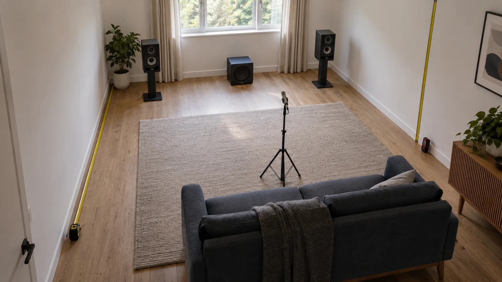
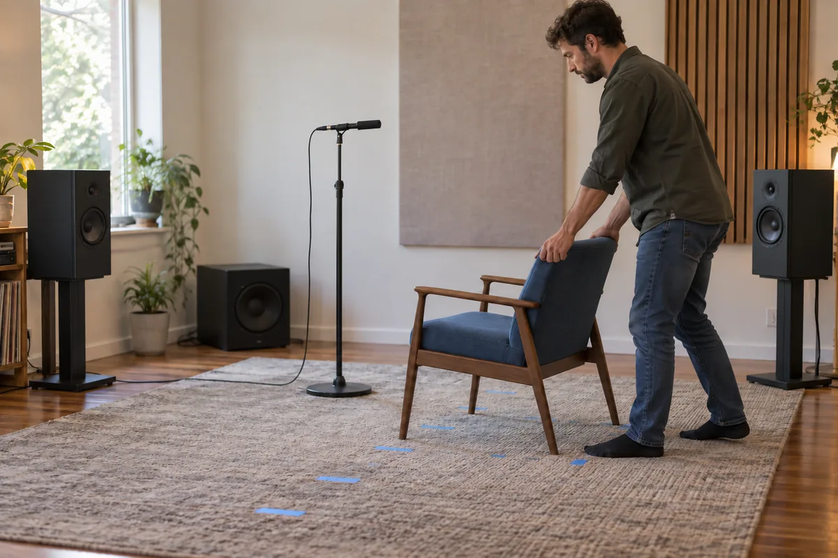
Use the same system state for every comparison: level, crossover, phase, delay, EQ, doors and major movable furnishings. Measure at ear height at the main position, then at nearby positions or other seats. Small spatial changes are valuable because modes create different pressure patterns across the room.
Compare the calculator with three views:
- Frequency response: Does a repeatable peak or dip occur near a predicted region?
- Spatial variation: Does it change substantially when the microphone moves?
- Decay: Does energy near that frequency persist longer than neighbouring frequencies?
Room EQ Wizard’s measurement primer explains that modal resonances appear as ridges that persist in a waterfall plot (REW). That time information matters: two peaks of similar height may require different priorities if one dies away quickly and the other rings audibly.
Turn Modal Clues Into Placement Decisions
Source position controls how strongly a mode is excited; listener position controls how that mode is sampled. Penn State’s room-mode demonstration shows that a source at a pressure antinode drives a mode strongly, while a source at a node may excite it very little (Penn State).
Start with reversible changes. Move the listening position forward or backward and repeat the sweep. Test speakers or a subwoofer at practical alternative positions, changing one variable at a time. Genelec likewise notes that moving monitors or the listening position can change how strongly room resonances appear (Genelec).
For a complete test sequence, continue with TFOOW’s subwoofer placement guide, including multi-seat measurements, crossover integration and deep-null limits.
When Multiple Subs, EQ, or Bass Traps Make Sense
The calculator alone cannot choose between these tools.
Multiple subwoofers are mainly a spatial-consistency strategy. Research by Todd Welti and Allan Devantier found that suitable multi-sub arrangements can reduce seat-to-seat low-frequency variation and make later equalisation more effective across a listening area (Audio Engineering Society). The finding does not mean that any two locations will work; measure each source and the combined system.
Equalisation can reduce a measured peak at relevant seats, but boosting a deep cancellation may waste headroom while barely filling the null. Fix position and integration first.
Bass trapping is a decay-control option when measurements show persistent low-frequency energy. A mode frequency can help define the region to investigate, but absorber type, depth, placement and boundary construction determine effectiveness. Thin broadband panels should not be assumed to control deep bass simply because the calculator identifies a low number.
What the Calculator Cannot Tell You
A basic room mode calculator assumes a closed rectangular volume with known dimensions and idealised boundaries. That is a defensible approximation for many bedrooms, studios and dedicated theatres, but its output becomes less literal when the space has:
- an open doorway into another volume;
- an L-shaped plan or several coupled rooms;
- a sloping ceiling or non-parallel boundaries;
- lightweight or flexible walls that absorb or transmit bass;
- large windows, doors, alcoves or built-in cavities;
- significant damping and furniture distributed unevenly;
- unknown construction behind the visible surfaces.
Even in a good rectangular case, the calculator does not predict the exact SPL at a seat, RT60, decay at every mode, speaker-boundary interference, crossover errors, distortion or rattles. More advanced finite-element or boundary-element models can represent complex geometry, but they still depend on accurate material and boundary data.
FAQ
Should I enter finished internal dimensions?
Yes. Measure the enclosed air volume between finished boundaries, not the building’s external dimensions. Use a consistent unit and include the actual finished ceiling height. If a recess or opening is large enough to behave as a coupled space, record it as a limitation rather than compressing the geometry into a misleading rectangle.
How close must a measured peak be to a calculated mode?
Do not require an exact match. Speed of sound, dimension uncertainty, boundary behaviour and frequency resolution all shift the comparison. Treat a calculated value as a nearby candidate, then check whether the measured response changes with position and whether decay data supports a resonance.
Can a room mode calculator find the best listening position automatically?
Not from dimensions alone. Some tools visualise ideal pressure patterns, which can suggest positions to test, but the best seat also depends on source locations, stereo symmetry, boundaries, crossover behaviour and the listening area. Use the result to narrow experiments, then measure the real system.
Conclusion
A room mode calculator is most valuable when it links dimensions to a disciplined measurement plan. Read axial modes first, flag clusters, gaps and coincidences, and use the Schroeder frequency only as an approximate regime boundary. Then test the predicted regions by moving the source and listener, measuring more than one position, and checking both response and decay.
If the real room disagrees with the model, trust repeatable measurements of the real room. The calculator’s job is to tell you where to look and which experiment to run next—not to replace that experiment.
Sources
- Jeffrey Hass, Indiana University. “Standing Waves and Room Modes.” Accessed September 28, 2026.
- MathWorks. “Compute Acoustic Room Transfer Function with Finite Element Analysis.” Accessed September 28, 2026.
- Daniel A. Russell, Pennsylvania State University. “Driving Room Modes: Source Location.”
- Room EQ Wizard. “Signals and Measurements.” Accessed September 28, 2026.
- Genelec. “How to Place Your Monitors.” Accessed September 28, 2026.
- Todd Welti and Allan Devantier. “Low-Frequency Optimization Using Multiple Subwoofers.” Journal of the Audio Engineering Society, May 2006.